This post is about a small project that I’ve been working on for the last month or so. I’ve been learning a lot about quantum computing lately, and as a theoretical undertaking that ties my research interests in math and physics with my more recent, practical computer-scientific adventures, the topic really excites me! The project concerns the quantum Schur transform (a quantum algorithm whose purpose I describe in a bit more detail in the Appendix) and consists in improvements to this Python implementation of a classical simulation of the version of the algorithm presented in this paper by Kirby and Strauch (the code is due to Kirby alone).
I came upon this algorithm because I was trying to spin up a version of another algorithm, the port-based teleportation protocols described in this paper, and the teleportation protocol requires the Schur transform as part of its construction. As I was toying with teleportation, I noticed somewhat slow runtimes of the Schur methods I was using, so I decided to peer under the hood and see what might be causing this. The main source of slow runtimes was the fact that Kirby used Python-native lists to represent the relevant unitary matrices, as opposed to NumPy or PyTorch. These modules are specifically optimized for matrix computations, so replacing Python lists and list comprehensions or for loops with equivalent numPy array or PyTorch methods leads to much faster run times. Further speedups were made possible by using PyTorch’s and sciPy’s sparse matrix implementations (many of the matrices acted as the identity on most of the qubits). The speedups obtained by my modifications are summarized by the following figure (note that the y-axis is on a logarithmic scale):
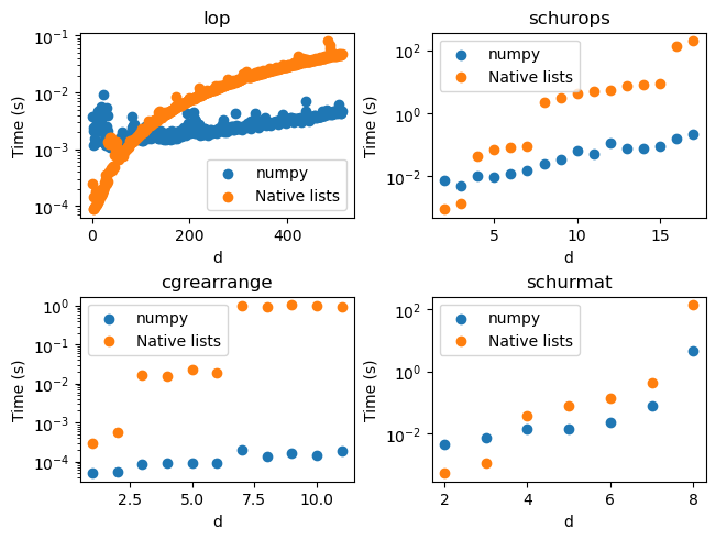
Each graph plots the average runtime for one iteration of an algorithm as a function of the natural parameter for that algorithm. The orange dots represent the original version of the algorithm, while the blue dots represent the new version. In the top-left graph, the size (side-length) of the relevant square matrices grows linearly with the parameter \(d\), whereas in the other graphs it grows exponentially; hence, for that method, I was able to get a better sense of the asymptotic behavior of both algorithms.
General Comments on the Graphs
In all four graphs, it’s clear that the asymptotic behavior of the NumPy-based algorithms is better than that of the original ones; in some concrete instances, the NumPy version outperformed the original by a factor of 5000! Another interesting general comment: there are noticeable jumps in runtime for the list-based algorithms at powers of two. I presume this has something to do with the dynamic sizing of Python-native lists.
Specific Comments on the Graphs
I turn now to each graph in turn. The top-left graph maps out how long it takes to construct the matrix of the lowering operator on a \(d\)-dimensional system. This is a square \(2d+1\)-matrix whose only non-zero entries are along the diagonal just above the main one. Hence, a sparse implementation of the function lop would be linear in \(d\); a dense implementation has complexity \(O(d^2)\). Indeed, this is what we see for the NumPy implementation. The original implementation builds up the matrix row-by-row, which requires periodically allocating more memory and copying the existing matrix. This leads to the worse asymptotic performance seen in the graph.
The bottom-left graph shows the implementations of a helper function; here were the greatest performance improvements, by a factor of 5000 or more.
The top-right graph shows one of the main functions, implementing a version of the Schur transform. Here and in the last graph, the greatest performance difference is the difference between minutes and seconds or fractions of a second.
Finally, the bottom-right graph shows the time it takes to compute the full unitary matrix for the Schur transform on \(d\) qubits. (This is the function which uses sparse PyTorch matrices.) The performance differences here are not as visually stark, but it should be noted that I was prevented from running the test for \(d=9\) and \(d=10\) by the slowness of the original algorithm, whereas the NumPy implementation could run in a feasible time on my machine. One-off tests for \(d=9\) yielded runtimes of 19 minutes and 13 seconds for the old and new implementations, respectively. Moreover, it is possible to run the schurmat function on a GPU (because it uses PyTorch matrix multiplication) and obtain even further speedups.
Conclusion This was a fun and practical exercise for me to get into the NumPy mindset. As a mathematician, I am used to thinking about matrix operations at a level of abstraction which is indifferent to the details of implementation. This project has helped me to get more in the computer scientist’s mindset: implementation can be the difference between a practical runtime and an impractical one!
Appendix: What is the Schur Transform?
For the interested reader, I want to briefly explain the purpose of the Schur transform. Given \(d\) qubits, let \(\sigma_{x,i}, \sigma_{y,i}, \sigma_{z,i}\) denote the matrices which act by
\[ \sigma_x = \begin{bmatrix} 0& 1\\ 1&0 \end{bmatrix}, \quad \sigma_y = \begin{bmatrix} 0 & -i\\ i & 0 \end{bmatrix}, \quad \sigma_z = \begin{bmatrix} 1 & 0 \\ 0 & -1 \end{bmatrix} \] respectively, on the \(i\)th qubit and otherwise by the identity. The computational basis is characterized by the fact that it is a set of joint eigenvectors for the \(d\) commuting operators \(\sigma_{z,1},\ldots \sigma_{z,d}\). A vector in the computational basis is uniquely and entirely determined by its eigenvalues for these \(d\) operators. The Schur transform takes the computational basis to the eigenbasis for a different commuting set of eigenvetors. Namely, let \[ S_{1,\ldots, j}= \left(\sum_{i=1}^j \sigma_{x,i}\right)^2 + \left(\sum_{i=1}^j \sigma_{y,i}\right)^2 + \left(\sum_{i=1}^j \sigma_{z,i}\right)^2 \] and let \[ Z = \sum_{i=1}^d \sigma_{z,i}. \] Then, the Schur basis is a basis of eigenvectors for the \(d\) commuting operators \((S_{1,2},S_{1,2,3},\ldots, S_{1,\ldots, d}, Z)\). Just as we had for the computational basis, a Schur basis vector is entirely and uniquely determined by its eigenvalues for these \(d\) operators. As mentioned above, the Schur transformation is simply the unitary transformation that takes the basis vectors of the computational basis to the basis vectors of the Schur basis (there is some confusion in the literature as to whether it is this matrix or its inverse/adjoint which is the true Schur transform).
The Schur basis is related to the representation theory of \(SU(2)\), which is deeply important in the mathematics of spin. But for the reader unfamiliar with representation theory, we can summarize the utility of the Schur basis by making the following observation: given an element \(v\) of the Schur basis, then for all \(i\), \(\sigma_{x,i}\cdot v\) (as well as \(\sigma_{y,i}\cdot v\) and \(\sigma_{z,i}\cdot v\)) will have the same eigenvalues for the \(S\) operators as \(v\) itself. (The same is not true for the computational basis, which gets shuffled around by the X and Y Pauli operators.) This can sometimes dramatically simplify the theoretical considerations involved in verifying the validity of a quantum protocol.